Gradient Descent
the Diploma thesis learning –
Machine learning has multiple methods to gradually improve solution by moving closer with intermediate result. One of more sophisticated methods is the Gradient Descent. Gradient descent is functional approach where you often approximate the result with some regard to difference of real (eg. measured) value and the predicted (function) value. In the statistics the difference is called error or the residual and is often used as cost function. The Gradient Descent tries to minimize the cost function.
There are two main types of functions – the loss function and the cost function. The loss function is function which displays the loss on one sample, one element, whereas the cost function is total of all the individual loss functions combined.
For example for linear regression we can use as cost function the Mean Squared Error (MSE). MSE displays how far from actual value the predicted value is. In other words how bad was the guess. The equation for Mean Squared Error is
(1) 
or vectorized ![]()
![]()
![]()
![]()
![]()
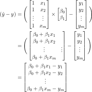
If we are looking on linear regression and our model ![]()
![]()
![]()
![]()
![]()
![]()
![]()
![]()
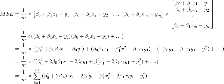
(2) 
Expanding the calculation based on ![]()
![]()
![]()
![]()
(3) 
where again ![]()
(4) 
The Mean Squared Errror is great in telling how far from real values our prediction is, but it has problem of not telling us which way to go (as it is squared, so it is always positive). That is why it is necessary to create partial derivation of MSE (gradient).
To simplify the equations we will halve the MSE. Using ![]() does not really matter as we are changing the cost function by a scalar while searching for the minimum of the function.
does not really matter as we are changing the cost function by a scalar while searching for the minimum of the function.
(5) 
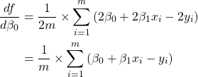
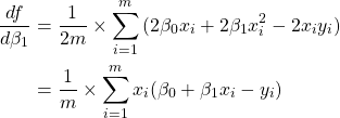
The cost function (in this case ![]() ) can be partially derived for each parameter of
) can be partially derived for each parameter of ![]() (in this case
(in this case ![]() ).
).
(6) 
(7) 
Using differentiation we can approach the local minimum using slope of the function (the slope is described by the first derivative). Having MSE function we can do partial derivation for each of the parameters and subtract the part of the slope of the previous solution to better approximate the function.
(8) 
Now having the partial derivatives it is time to use them to improve the parameters. Only thing remaining is choosing the correct step size ![]() . It is important to choose proper size. Choose too big steps and it would mean jumping too far a back. Choose too small step size and it will take close to infinite amount of time to improve the parameters.. Often simple 1% change (
. It is important to choose proper size. Choose too big steps and it would mean jumping too far a back. Choose too small step size and it will take close to infinite amount of time to improve the parameters.. Often simple 1% change (![]() ) in time seems like a good fit as it is simple enough to not complicate the counting yet big enough to make change in time.
) in time seems like a good fit as it is simple enough to not complicate the counting yet big enough to make change in time.
(9) 
And this is one iteration of Gradient Descent. Now few hundred, maybe thousands (depending on model and initial guess), to converge to local minimum.